Spider Plot

Last updated on Aug 26, 2026 6 min read

Table of Contents

⚠️ Make Sure You Understand the Code Before Using It ⚠️

Introduction

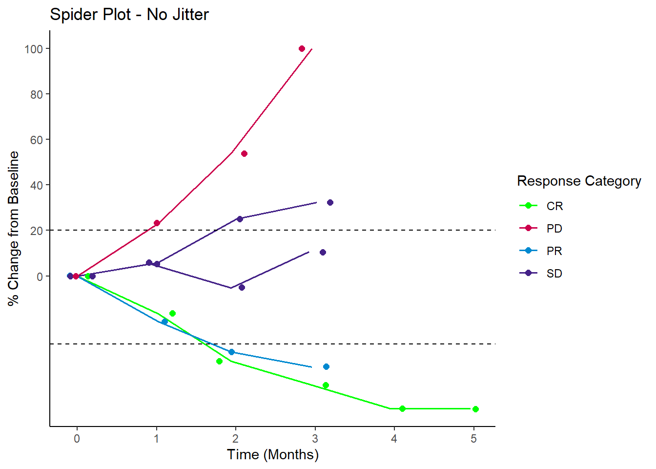
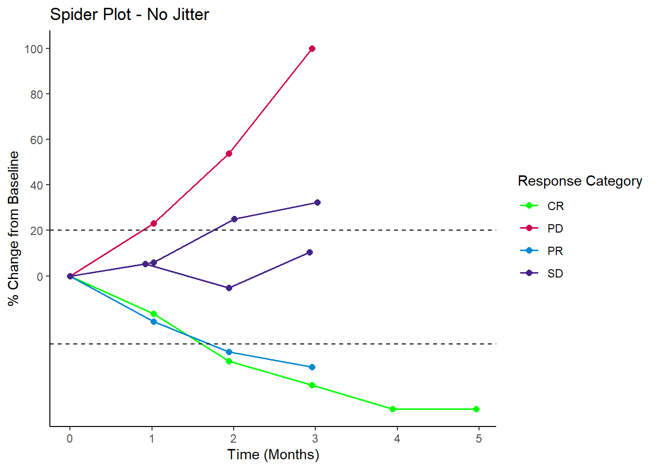
A function to generate a spider plot showing longitudinal changes over time for each individual, commonly used to visualize tumor response or biomarker changes in oncology trials.

Input

data: Longitudinal data with one row per individual per timepoint
x_var: X-axis variable column name (string, e.g., “Time”)
y_var: Y-axis variable column name (string, e.g., “pct_change”)
id_var: ID column name (string)
group_var: Optional grouping variable for colors (string)
reference_lines: Optional numeric vector for horizontal reference lines
title: Plot title (string)
xlab: X-axis label (string)
ylab: Y-axis label (string)
y_breaks: Y-axis breaks (e.g., seq(0, 20, by = 2))
x_breaks: X-axis breaks (e.g., seq(0, 20, by = 2))
color_palette: Optional named vector of colors for groups
legend_title: Legend title (string)
point_size: Size of points (numeric, default 2)
line_width: Width of lines (numeric, default 0.6)
jitter: Whether to jitter points (logical, default FALSE)
jitter_width: Width of jitter for points (numeric, default 0.1)
legend_position: Legend position (numeric vector c(x, y) or string like “bottom”, “right”, “none”)
legend_title_size: Legend title size (numeric)
legend_text_size: Legend text size (numeric)
axis_text_size: Axis ticks text size (numeric)
axis_title_size: Axis label text size (numeric)
x_angle: X-axis text rotation angle (numeric, e.g., -30)

Output

A ggplot2 object

Example Data

library(dplyr)
library(ggplot2)

# Example raw longitudinal data
raw_data <- tribble(
  ~ID, ~date_lab, ~lab_value, ~cycle, ~treatment_arm, ~response_category, ~end_date,
  
  "PT001", "2023-01-01", 50, "Screening", "Arm A", "CR", "2023-12-31",
  "PT001", "2023-01-15", 48, "Cycle 1", "Arm A", "CR", "2023-12-31",
  "PT001", "2023-02-15", 40, "Cycle 2", "Arm A", "CR", "2023-12-31",
  "PT001", "2023-03-15", 30, "Cycle 3", "Arm A", "CR", "2023-12-31",
  "PT001", "2023-04-15", 25, "Cycle 4", "Arm A", "CR", "2023-12-31",
  "PT001", "2023-05-15", 20, "Cycle 5", "Arm A", "CR", "2023-12-31",
  "PT001", "2023-06-15", 20, "Off Treatment", "Arm A", "CR", "2023-12-31",
  
  "PT002", "2023-01-05", 80, "Screening", "Arm B", "PR", "2023-12-31",
  "PT002", "2023-01-20", 75, "Cycle 1", "Arm B","PR", "2023-12-31",
  "PT002", "2023-02-20", 60, "Cycle 2", "Arm B","PR", "2023-12-31",
  "PT002", "2023-03-20", 50, "Cycle 3", "Arm B","PR", "2023-12-31",
  "PT002", "2023-04-20", 45, "Cycle 4", "Arm B","PR", "2023-12-31",
  
  "PT003", "2023-02-01", 100, "Screening", "Arm A", "SD", "2023-12-31",
  "PT003", "2023-02-15", 95, "Cycle 1", "Arm A", "SD", "2023-12-31",
  "PT003", "2023-03-15", 100, "Cycle 2", "Arm A", "SD", "2023-12-31",
  "PT003", "2023-04-15", 90, "Cycle 3", "Arm A", "SD", "2023-12-31",
  "PT003", "2023-05-15", 105, "Cycle 4", "Arm A", "SD", "2023-12-31",
  
  "PT004", "2023-01-10", 60, "Screening", "Arm B", "PD", "2023-12-31",
  "PT004", "2023-01-25", 65, "Cycle 1", "Arm B", "PD", "2023-12-31",
  "PT004", "2023-02-25", 80, "Cycle 2", "Arm B", "PD", "2023-12-31",
  "PT004", "2023-03-25", 100, "Cycle 3", "Arm B", "PD", "2023-12-31",
  "PT004", "2023-04-25", 130, "Cycle 4", "Arm B", "PD", "2023-12-31",
  
  "PT005", "2023-03-01", 70, "Screening", "Arm A", "SD", "2023-05-01",
  "PT005", "2023-03-15", 68, "Cycle 1", "Arm A", "SD", "2023-05-01",
  "PT005", "2023-04-15", 72, "Cycle 2", "Arm A", "SD", "2023-05-01",
  "PT005", "2023-05-15", 85, "Cycle 3", "Arm A", "SD", "2023-05-01",
  "PT005", "2023-06-15", 90, "Cycle 4", "Arm A", "SD", "2023-05-01"
)

Example Data Wrangling

spider_data = 
  raw_data %>% 
  mutate(
    date_lab = as.Date(date_lab),
    end_date = as.Date(end_date), # If any data cut-off date
    cycle_reorder = factor(cycle, levels = c("Screening", paste("Cycle", 1:5), "Off Treatment"))) %>% # edit based on your data
  relocate(cycle_reorder, .after = cycle) %>%
  group_by(ID) %>%
  arrange(ID, date_lab, cycle_reorder) %>%
  mutate(
    ## calculate time elapsed (months) from the start of treatment (cycle 1) to the date of each lab measure, start date could also be screening, depends on the design
    date_elapsed_days = as.numeric(date_lab - date_lab[cycle == "Cycle 1"]),
    date_elapsed_months = as.numeric(date_elapsed_days / 30.437),
    

    ## calculate % change in lab measure from the start of treatment (cycle 1)
    from_cycle1_pct = ifelse(
      cycle == "Screening", 
      NA_real_,
      (lab_value - lab_value[cycle == "Cycle 1"])/lab_value[cycle == "Cycle 1"] * 100
    ),    
  ) %>%
  relocate(from_cycle1_pct, .before = lab_value) %>%
  select(
    ID, 
    date_lab, date_elapsed_days, date_elapsed_months,
    cycle, cycle_reorder, lab_value, from_cycle1_pct, response_category, end_date
  ) %>%
  
  ## filtering data for spider plot
  filter(cycle != "Screening")

# ## data checking
# test = spider_data %>% filter(Cycle == "Cycle 1")
# sum(test$date_lab == test$start_date)
spider_end_date = spider_data %>% filter(date_lab <= end_date)

Function

spider_plot <- function(
    data,
    x_var,
    y_var,
    id_var = "ID",
    group_var = NULL,
    reference_lines = NULL,
    title = NULL,
    xlab = "X-axis",
    ylab = "Y-axis",
    y_breaks = NULL,
    x_breaks = NULL,
    color_palette = NULL,
    legend_title = NULL,
    point_size = 2,
    line_width = 0.6,
    jitter = FALSE,
    jitter_width = 0.1,
    legend_position = NULL,
    legend_title_size = NULL,
    legend_text_size = NULL,
    axis_text_size = NULL,
    axis_title_size = NULL,
    x_angle = NULL
){
  
  # Create internal variables
  data$x <- data[[x_var]]
  data$y <- data[[y_var]]
  data$id <- data[[id_var]]
  
  # Add group variable if provided
  if (!is.null(group_var)) {
    data$group <- data[[group_var]]
  }
  
  # Set legend title (use group_var if legend_title not provided)
  if (is.null(legend_title) & !is.null(group_var)) {
    legend_title <- group_var
  }
  
  # Base plot
  if (!is.null(group_var)) {
    p <- ggplot(data, aes(x = x, y = y, group = id, color = group))
  } else {
    p <- ggplot(data, aes(x = x, y = y, group = id))
  }
  
  # Add lines
  p <- p + geom_line(linewidth = line_width)
  
  # Add points with or without jitter
  if (jitter) {
    p <- p + geom_point(size = point_size, position = position_jitter(width = jitter_width))
  } else {
    p <- p + geom_point(size = point_size)
  }
  
  # Add reference lines
  if (!is.null(reference_lines)) {
    for (ref in reference_lines) {
      p <- p + geom_hline(yintercept = ref, linetype = "dashed")
    }
  }
  
  
  # Add labels
  p <- p +
    labs(
      title = title,
      x = xlab,
      y = ylab,
      color = legend_title
    )
  
  # Add y-axis breaks if provided
  if (!is.null(y_breaks)) {
    p <- p + scale_y_continuous(breaks = y_breaks)
  }
  
  # Add x-axis breaks if provided
  if (!is.null(x_breaks)) {
    p <- p + scale_x_continuous(breaks = x_breaks)
  }
  
  # Add custom color palette if provided
  if (!is.null(group_var) & !is.null(color_palette)) {
    p <- p + scale_color_manual(values = color_palette)
  }
  
  # Apply theme
  p <- p + theme_classic()
  
  # Build theme modifications
  theme_mods <- list()
  
  if (!is.null(legend_position)) {
    theme_mods$legend.position <- legend_position
  }
  
  if (!is.null(legend_title_size)) {
    theme_mods$legend.title <- element_text(size = legend_title_size)
  }
  
  if (!is.null(legend_text_size)) {
    theme_mods$legend.text <- element_text(size = legend_text_size)
  }
  
  if (!is.null(axis_text_size)) {
    theme_mods$axis.text <- element_text(size = axis_text_size)
  }
  
  if (!is.null(axis_title_size)) {
    theme_mods$axis.title <- element_text(size = axis_title_size)
  }
  
  if (!is.null(x_angle)) {
    theme_mods$axis.text.x <- element_text(angle = x_angle, hjust = 1, vjust = -0.5)
  }
  
  # Apply theme modifications if any
  if (length(theme_mods) > 0) {
    p <- p + do.call(theme, theme_mods)
  }
  
  return(p)
}

Plot Without jitter

plot_no_jitter <- spider_plot(
  data = spider_data,
  x_var = "date_elapsed_months",
  y_var = "from_cycle1_pct",
  id_var = "ID",
  group_var = "response_category",
  reference_lines = c(-30, 20),
  title = "Spider Plot - No Jitter",
  xlab = "Time (Months)",
  ylab = "% Change from Baseline",
  y_breaks = seq(0, 140, 20),
  x_breaks = seq(0, 5, 1),
  color_palette = c("CR" = "green", "PR" = "#0089D0", "SD" = "#442288", "PD" = "#CC004C"),
  legend_title = "Response Category",
  jitter = FALSE
)

Plot With jitter

plot_with_jitter <- spider_plot(
  data = spider_data,
  x_var = "date_elapsed_months",
  y_var = "from_cycle1_pct",
  id_var = "ID",
  group_var = "response_category",
  reference_lines = c(-30, 20),
  title = "Spider Plot - No Jitter",
  xlab = "Time (Months)",
  ylab = "% Change from Baseline",
  y_breaks = seq(0, 140, 20),
  x_breaks = seq(0, 5, 1),
  color_palette = c("CR" = "green", "PR" = "#0089D0", "SD" = "#442288", "PD" = "#CC004C"),
  legend_title = "Response Category",
  jitter = TRUE,
  jitter_width = 0.2
)

R Code Figure